Variational Auto-Encoder
In an inference problem, $p(z\vert x)$, which is used to infer $z$ from $x$.
$$ p(z\vert x) = \frac{p(x, z)}{p(x)}. $$
For example, we have an observable $x$ and a latent space $z$, we would like to find a good latent space for the observable $x$. However, $p(x)$ is something we don’t really know. We would like to use some simpler quantities to help us inferring $z$ from $x$ or generating $x$ from $z$.
Now we introduce a simple distribution $q(z\vert x)$. We want to make sure this $q(z\vert x)$ is doing a good job of replacing $p(z\vert x)$, i.e., minimizing the [[KL divergence]] KL Divergence Kullback–Leibler divergence indicates the differences between two distributions ,
$$ \operatorname{min}_{q(z\vert x)} \operatorname{KL} (q(z\vert x) \parallel p(z\vert x)). $$
We can reformulate this KL divergence
$$ \begin{align*} & \operatorname{KL} (q(z\vert x) \parallel p(z\vert x)) \\ =& -\sum_{z} q(z\vert x) \ln \frac{ p(z\vert x) }{ q(z\vert x) } \\ =& -\sum_{z} q(z\vert x) \left( \ln \frac{ p(x, z) }{ q(z\vert x) } - \ln p(x) \right) \\ =& -\sum_{z} q(z\vert x) \ln \frac{ p(x, z) }{ q(z\vert x) } + \sum_{z} q(z\vert x) \ln p(x) \\ =& -\sum_{z} q(z\vert x) \ln \frac{ p(x, z) }{ q(z\vert x) } + \ln p(x) {\color{red}\sum_{z} q(z\vert x)} \\ =& -\sum_{z} q(z\vert x) \ln \frac{ p(x, z) }{ q(z\vert x) } + \ln p(x) \end{align*} $$
where we have used ${\color{red}\sum_{z} q(z\vert x)}=1$.
Rewriting the above
$$ \ln p(x) = \operatorname{KL} ( q(z\vert x) \parallel p(z\vert x) ) + {\color{blue}\sum_z q(z) \ln \frac{p(x, z)}{q(z\vert x)}}, $$
where we define
$$ \mathcal L \equiv {\color{blue}\sum_z q(z) \ln \frac{p(x, z)}{q(z\vert x)}} $$
as the so called [[Evidence Lower Bound (ELBO)]] Evidence Lower Bound: ELBO ELBO is an very important concept in variational methods .
We want to minimize $\operatorname{KL} ( q(z\vert x) \parallel p(z\vert x) )$. Since $\ln p(x)$ should be a fixed number given an observation, we can maximize $\mathcal L$. We also know that the KL divergence is non-negative, we get
$$ \mathcal L \leq \ln p(x). $$
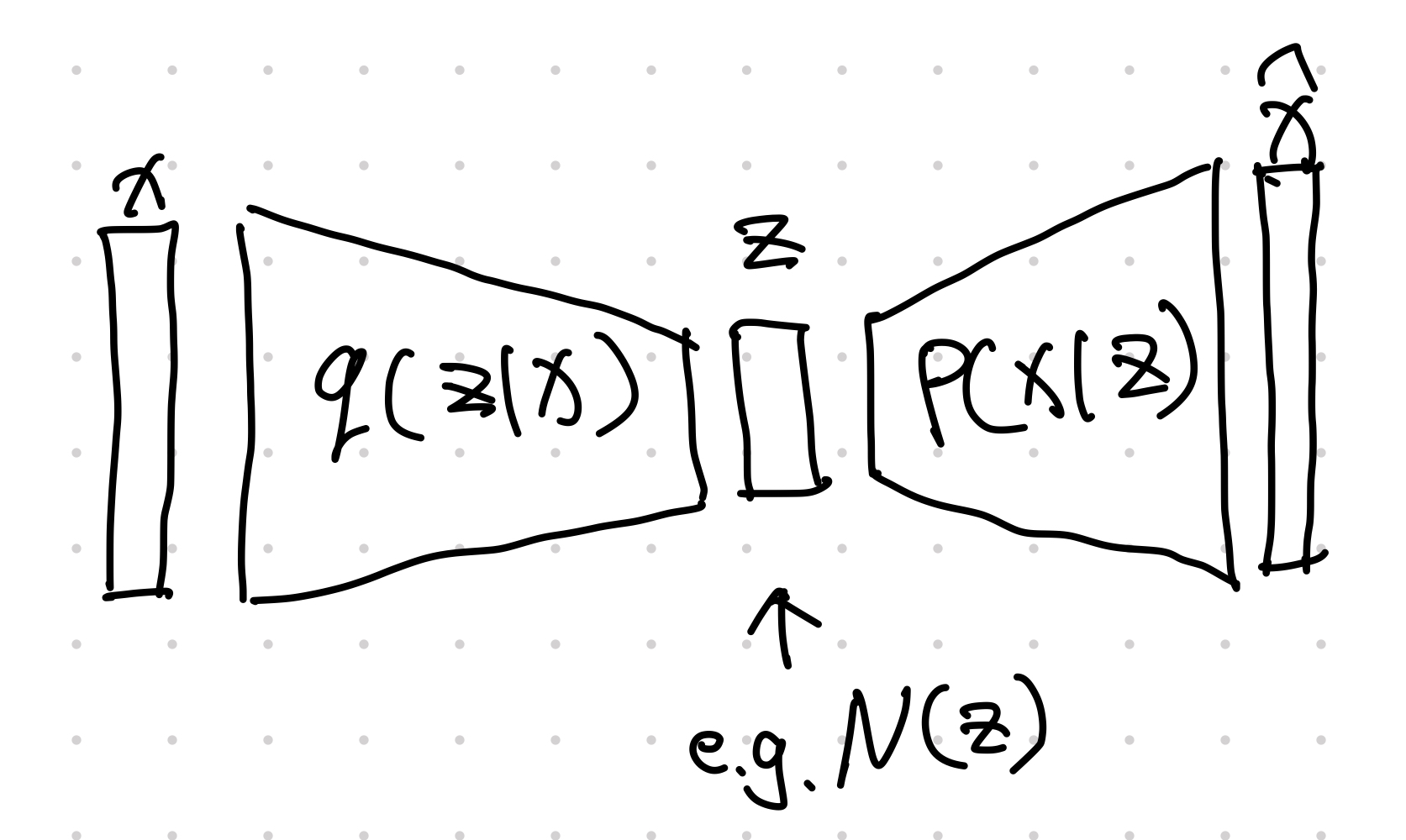
To map our method to an encoder decoder structure, we rewrite $\mathcal L$,
$$ \begin{align} \mathcal L =& \sum_z q(z\vert x) \ln \frac{p(x,z)}{q(z\vert x)} \\ =& \sum_z q(z\vert x) \ln \frac{p(x\vert z)p(z)}{q(z\vert x)} \\ =& \sum_z q(z\vert x) \left( \ln p(x\vert z) + \ln\frac{p(z)}{q(z\vert x)} \right) \\ =& \sum_z q(z\vert x) \ln p(x\vert z) + \sum_z q(z\vert x) \ln \frac{p(z)}{q(z\vert x)} \\ =& \mathbb E_{q(z\vert x)}\ln p(x\vert z) - \operatorname{KL}( q(z\vert x) \parallel p(z) ). \end{align} $$
With the above equation, we can map the quantities to an encoder-decoder structure.
An Alternative View
Variational Auto-Encoder (VAE) is very different from [[Generative Model: Auto-Encoder]] Generative Model: Auto-Encoder Autoencoders (AE) are machines that encodes inputs into a compact latent space. The simplest auto-encoder is rather easy to understand. The loss can be chosen based on the demand, e.g., cross entropy for binary labels. Notation: dot ($\cdot$) We use a single vertically centered dot, i.e., $\cdot$, to indicate that the function or machine can take in arguments. A simple autoencoder can be achieved using two neural nets, e.g., $$ \begin{align} {\color{green}h} &= … . In VAE, we introduce a variational distribution $q$ to help us work out the weighted integral after introducing the latent space variable $z$,1
$$ \begin{align} \ln p_\theta(x) &\geq \int \left(\ln p_\theta (x\mid z) \right)p(z) \,\mathrm d z \\ &= \int \left(\ln\left(\frac{q_{\phi}(z\mid x)}{q_{\phi}(z\mid x)} p_\theta (x\mid z)\right) \right) p(z) \, \mathrm d z \end{align} $$
where the first line is obtained from the [[Jensen's Inequality]] Jensen's Inequality Jensen’s inequality shows that $$ f(\mathbb E(X)) \leq \mathbb E(f(X)) $$ for a concave function $f(\cdot)$. (see derivation in [[Evidence Lower Bound: ELBO]] Evidence Lower Bound: ELBO ELBO is an very important concept in variational methods ).
In the above derivation,
- ${}_\theta$ is the model for inference, and
- ${}_\phi$ is the model for variational approximation.
![From simple distribution in latent space to a more complex distribution. [Doersch2016]](../assets/generative-variational-autoencoder/1606.05908-fig2-gaussian-latent.png)
From simple distribution in latent space to a more complex distribution. [Doersch2016]
The demo looks great. However, sampling from latent space becomes more difficult as the dimension of the latent space increases. We need a more efficient way to sample from the latent space. One solution is to apply the variational method. To to sample $z$, the method uses a model that samples $z$ based on $x$, i.e., introduce a function $q(z\mid x)$ to help us with sampling in latent space.
$$ \begin{align} \ln p_\theta(x) &= \int \left(\ln p_\theta (x\mid z) \right)p(z) \,\mathrm d z \\ &= \int \left(\ln\frac{q_{\phi}(z\mid x)}{q_{\phi}(z\mid x)} p_\theta (x\mid z) \right) p(z) \, \mathrm d z \\ &= \int \left(\ln\frac{q_{\phi}(z\mid x)}{q_{\phi}(z\mid x)} \frac{p_\theta (x, z)}{p (z)} \right) p(z) \, \mathrm d z \\ &= \int dz q(z\mid x) \ln \frac{p(x,z)}{q(z\mid x)} + \int dz q(z\mid x) \ln \frac{q(z\mid x)}{p(z\mid x)} \label{eqn-vae-lnp-sep-q} \\ &= - \left[ D_{\mathrm{KL}} ( q_{\phi}(z\mid x) \mathrel{\Vert} p(z) ) - \mathbb E_q ( \ln p_\theta (x\mid z) ) \right] + D_{\mathrm{KL}}( q(z\mid x)\parallel p(z\mid x) ) \label{eqn-vae-lnp-decompositions} \\ & \geq - \left[ D_{\mathrm{KL}} ( q_{\phi}(z\mid x) \mathrel{\Vert} p(z) ) - \mathbb E_q ( \ln p_\theta (x\mid z) ) \right] \label{eqn-vae-lnp-geq-elbo} \\ &\equiv - F(x) \\ &\equiv \mathcal L . \end{align} $$
In the derivation, the row ($\ref{eqn-vae-lnp-sep-q}$) is validate because $\int dz q(z\mid x) = 1$.
The term $F(x)$ is the free energy, while the negative of it, $-F(x)=\mathcal L$, is the so-called [[Evidence Lower Bound (ELBO)]] Evidence Lower Bound: ELBO ELBO is an very important concept in variational methods ,
$$ \mathcal L = - D_{\mathrm{KL}} ( q_{\phi}(z\mid x) \mathrel{\Vert} p(z) ) + \mathbb E_q ( \ln p_\theta (x\mid z) ). $$
From row ($\ref{eqn-vae-lnp-decompositions}$) to ($\ref{eqn-vae-lnp-geq-elbo}$), we dropped the term $D_{\mathrm{KL}}( q(z\mid x)\parallel p(z\mid x) )$ which is always nonnegative. The reason is that we can not maximize this [[KL divergence]] KL Divergence Kullback–Leibler divergence indicates the differences between two distributions as we do not know $p(z\mid x)$. But the KL divergence is always non-negative. So if we find a $q$ that can maximize $\mathcal L$, then we are also miminizing the KL divergence (with a function $q(z\mid x)$ that is close to $p(z\mid x)$) and maximizing the loglikelihood loss. Now we only need to find a way to maximize $\mathcal L$.
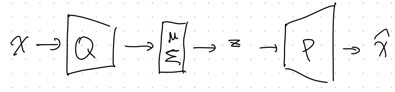
Using Neural networks
We model the parameters of the Gaussian distribution $p_\theta(x\mid z)$, e.g., $f(z, \theta)$, using a neural network.
In reality, we choose a gaussian form of the variational functional with the mean and variance depends on the data $x$ and the latent variable $z$
$$ q(z\mid x) = \mathcal N ( \mu(x,z), \Sigma (x,z) ). $$
We have
$$ \begin{align} &\ln p_\theta(x\mid z) \\ =& \ln \mathscr N( x\mid f(z, \theta), \sigma^2 I )\\ =& \ln \left( \frac{1}{\sqrt{2\pi \sigma^2}} \exp{\left( -\frac{(x -f(z,\theta)^2)}{\sigma^2} \right)} \right) \\ =& -(x - f(z, \theta))^2 + \mathrm{Const.} \end{align} $$
Why don’t we simply draw $q$ from $p(z)$?
Structure
Structure of VAE
Doersch wrote a very nice tutorial on VAE2. We can find the detailed structures of VAE.
Another key component of VAE is the [[reparametrization trick]] Reparametrization in Expectation Sampling Reparametrize the sampling distribution to simplify the sampling . The variational approximation $q_\phi$ is usually a Gaussian distribution. Once we get the parameters for the Gaussian distribution, we will have to sample from the Gaussian distribution based on the parameters. However, this sampling process prohibits us from propagating errors. The [[reparametrization trick]] Reparametrization in Expectation Sampling Reparametrize the sampling distribution to simplify the sampling solves this problem.
Loss Explanation
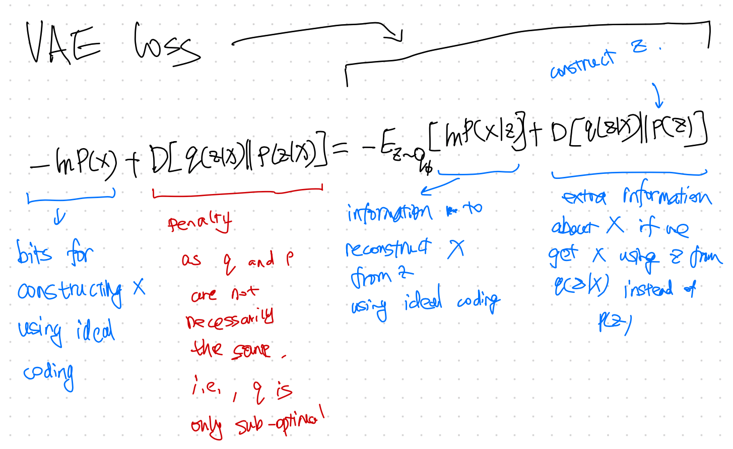
VAE Loss Explained
- Liu2020 Liu X, Zhang F, Hou Z, Wang Z, Mian L, Zhang J, et al. Self-supervised Learning: Generative or Contrastive. arXiv [cs.LG]. 2020. Available: http://arxiv.org/abs/2006.08218
- Doersch2016 Doersch C. Tutorial on Variational Autoencoders. arXiv [stat.ML]. 2016. Available: http://arxiv.org/abs/1606.05908
- Kingma2019 Kingma DP, Welling M. An Introduction to Variational Autoencoders. arXiv [cs.LG]. 2019. Available: http://arxiv.org/abs/1906.02691
- Jordan J. Variational autoencoders. Jeremy Jordan. 19 Mar 2018. Available: https://www.jeremyjordan.me/variational-autoencoders/. Accessed 22 Aug 2021.
- Courses DS. Ali Ghodsi, Lec : Deep Learning, Variational Autoencoder, Oct 12 2017 [Lect 6.2]. YouTube. 2017. Available: https://youtu.be/uaaqyVS9-rM?t=19m42s
wiki/machine-learning/generative-models/variational-autoencoder:wiki/machine-learning/generative-models/variational-autoencoder Links to:L Ma (2021). 'Variational Auto-Encoder', Datumorphism, 08 April. Available at: https://datumorphism.leima.is/wiki/machine-learning/generative-models/variational-autoencoder/.