Generative Model: Normalizing Flow

Normalizing flow is a method to convert a complicated distribution $p(x)$ to a simpler distribution $\tilde p(z)$ by building up a map $z=f(y)$ for the variable $x$ to $z$. The relations between the two distributions is established using the conservation law for distributions, $\int p(x) \mathrm d x = \int \tilde p (z) \mathrm d z = 1$. One could imagine that changing the variable also brings in the Jacobian.

Architecture

For a probability density $p(x)$ and a transformation of coordinate $x=g(z)$ or $z=f(x)$, the density can be expressed using the coordinate transformations, i.e.,¹

$$ \begin{align} p(x) &= \tilde p (f(x)) \lvert \operatorname{det} \operatorname{D} g(f(x)) \rvert^{-1} \\ &= \tilde p(f(x)) \lvert \operatorname{det}\operatorname{D} f(x) \rvert \end{align} $$

where the Jacobian is

$$ \operatorname{D} g(z) \to \frac{\partial }{\partial z} g. $$

The operation $g _ { * }\circ \tilde p(z)$ is the pushforward of $\tilde p(z)$. The operation $g _ { * }$ will pushforward simple distribution $\tilde p(z)$ to a more complex distribution $p(x)$.

• The generative direction: sample $z$ from distribution $\tilde p(z)$, apply transformation $g(z)$;
• The normalizing direction: “simplify” $p(x)$ to some simple distribution $\tilde p(z)$.

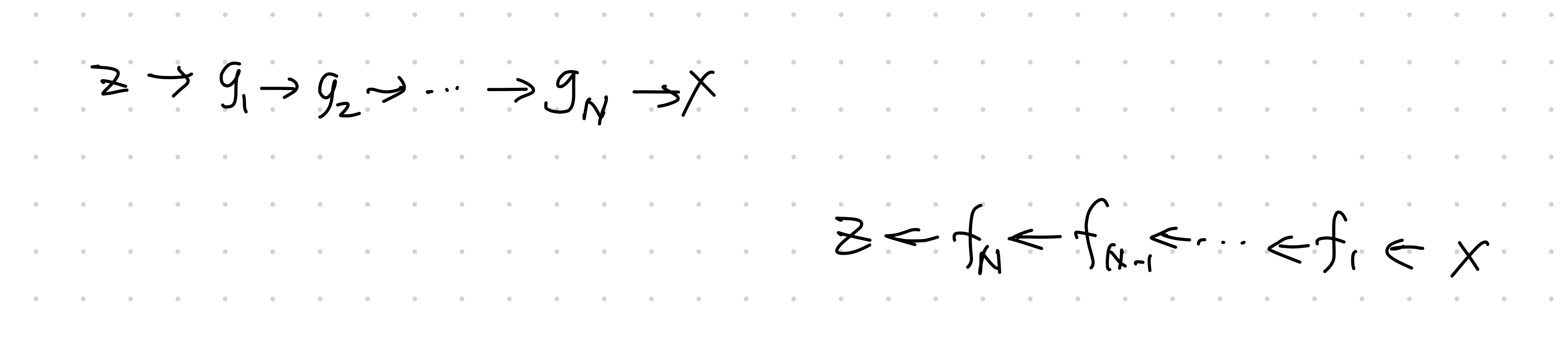
The key to the flow model is the chaining of the transformations

$$ \operatorname{det} \operatorname{D} f(x) = \Pi_{i=1}^N \operatorname{det} \operatorname{D} f_i (x_i) $$

where

$$ \begin{align} x_i &= g_i \circ \cdots \circ g_1 (z)\\ &= f_{i+1} \circ \cdots \circ f_N (x). \end{align} $$

Applications

Normalizing flow is good at estimating densities, fast.¹

Variational Inference

One interesting use case of the normalizing flow model is variational inference. We reiterate section 2.2.2 of Liu2020 here.¹

• The variational inference problem: $\ln p(x) = \int \ln p(x, y) dy = $:
  • $x$ is the observable;
  • $y$ is the latent variable.
• Introduce an approximation of the posterior $q(y\vert x, \theta)$, see