Autoregressive Denoising Diffusion Model

Autoregressive

In an multivariate [[forecasting problem]] The Time Series Forecasting Problem Forecasting time series , given an input sequence $\mathbf x_{t-K: t}$, we forecast $\mathbf x_{t+1:t+H}$.

To apply the [[denoising diffusion model]] Diffusion Models for Forecasting Objective In a denoising diffusion model, given an input $\mathbf x^0$ drawn from a complicated and unknown distribution $q(\mathbf x^0)$, we find a latent space with a simple and manageable distribution, e.g., normal distribution, and the transformations from $\mathbf x^0$ to $\mathbf x^n$, as well as the transformations from $\mathbf x^n$ to $\mathbf x^0$. An Example For example, with $N=5$, the forward process is flowchart LR x0 --> x1 --> x2 --> x3 --> x4 --> x5 and the reverse process is … in our multivariate forecasting problem, we define our forecasting task as an autoregressive problem

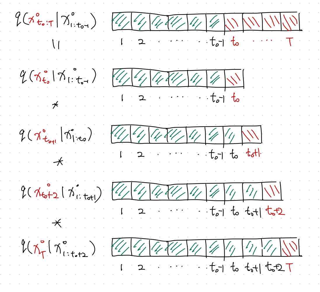
$$ q(\mathbf x^0_{t - K:t} \vert \mathbf x^0_{1:t_0 - 1}) = \Pi_{t=t_0}^T q(\mathbf x^0_t \vert \mathbf x^0_{1:t-1}). $$

Time Dynamics

Time dynamics can be easily captured by some RNN, meanwhile, we need a model for the diffusion process at each time step. Note that in [[denoising diffusion model]] Diffusion Models for Forecasting Objective In a denoising diffusion model, given an input $\mathbf x^0$ drawn from a complicated and unknown distribution $q(\mathbf x^0)$, we find a latent space with a simple and manageable distribution, e.g., normal distribution, and the transformations from $\mathbf x^0$ to $\mathbf x^n$, as well as the transformations from $\mathbf x^n$ to $\mathbf x^0$. An Example For example, with $N=5$, the forward process is flowchart LR x0 --> x1 --> x2 --> x3 --> x4 --> x5 and the reverse process is … , we minimize

$$ \operatorname{min}_\theta \mathbb E_{q(\mathbf x^0)} \left[ -\log p_\theta (\mathbf x^0) \right] $$

The above loss becomes that of the denoising model for a single time step. Explicitly,

$$ \operatorname{min}_\theta \mathbb E_{q(\mathbf x^0_t )} \left[ -\log p_\theta (\mathbf x^0_t) \right]. $$

To include the time dynamics, we use the RNN state of the previous time step $\mathbf h_{t-1}$¹

$$ \operatorname{min}_\theta \mathbb E_{q(\mathbf x^0_t )} \left[ -\log p_\theta (\mathbf x^0_t \vert \mathbf h_{t-1}) \right]. $$

Apart from the usual time dimension $t$, the autoregressive denoising diffusion model has another dimension to optimize: the diffusion step $n$ for each time $t$.

The loss for each time step $t$ is¹

$$ \mathcal L_t = \mathbb E_{\mathbf x^0_t, \epsilon, n} \left[ \lVert \epsilon - \epsilon_\theta ( \sqrt{\bar \alpha_n} \mathbf x^0_t + \sqrt{1-\bar \alpha_n}\epsilon, \mathbf h_{t-1}, n ) \rVert^2 \right]. $$

That being said, we just need to minimize $\mathcal L_t$ for each time step $t$.

Training Algorithm

See Rasul et al., (2021)¹.

How to Forecast

After training, we obtain the time dynamics encoding $\mathbf h_T$, with which the denoising steps can be calculated using the reverse process

$$ \mathbf x^{n-1}_{T+1} = \frac{1}{\alpha_n} \left( \mathbf x^n_{T+1} - \frac{\beta_n}{1 - \bar\alpha_n} \epsilon_\theta( \mathbf x^n_{T+1}, \mathbf h_{T}, n ) \right) + \sqrt{\Sigma_\theta} \mathbf z, $$

where $\mathbf z \sim \mathcal N(\mathbf 0, \mathbf I)$.

For example,

$$ \mathbf x^{0}_{T+1} = \frac{1}{\alpha_1} \left( \mathbf x^1_{T+1} - \frac{\beta_1}{1 - \bar\alpha_1} \epsilon_\theta( \mathbf x^1_{T+1}, \mathbf h_{T}, 1 ) \right) + \sqrt{\Sigma_\theta} \mathbf z. $$

It is Probabilistic

The quantiles is calculated by repeating many times for each forecasted time step¹.