Conformal Prediction
Conformal prediction is a method to predict a consistent confidence interval in an on-line setting. The algorithms is following the [[Neyman-Pearson hypothesis testing]] Neyman-Pearson Theory The Neyman-Pearson hypothesis testing tests two hypothesis, hypothesis $H$, and an alternative hypothesis $H_A$. Neyman-Pearson Lemma The Neyman-Pearson Lemma is an very intuitive lemma to understand how to choose a hypothesis. The lecture notes from PennState is a very good read on this topic1. An example For simplicity, we assume that there exists a test statistic $T$ and $T$ can be used to measure how likely the hypothesis $H$ is true, e.g., the hypothesis $H$ is false, corresponds to $T$ … framework, thus providing solid theoretical support for the predicted region.
Nonconformity Measure
For a new incoming data point $x$, and an existing [[multiset]] Multiset, mset or bag A bag is a set in which duplicate elements are allowed. An ordered bag is a list that we use in programming. of data points
$$ B_n = \{\!\{x_1, \cdots, x_{n}\}\!\}, $$
a nonconformity measure, $A(B_n, x)$, measures how different $x_n$ is from the existing multiset1.
A naive choice would be to reuse our model $x = f(B_n)$. Define a nonconformity measure
$$ A(B_n, x) = d(f(B_n), x), $$
where $d$ is some kind of [[Distance]] Distance .
A Conformal Algorithm Example
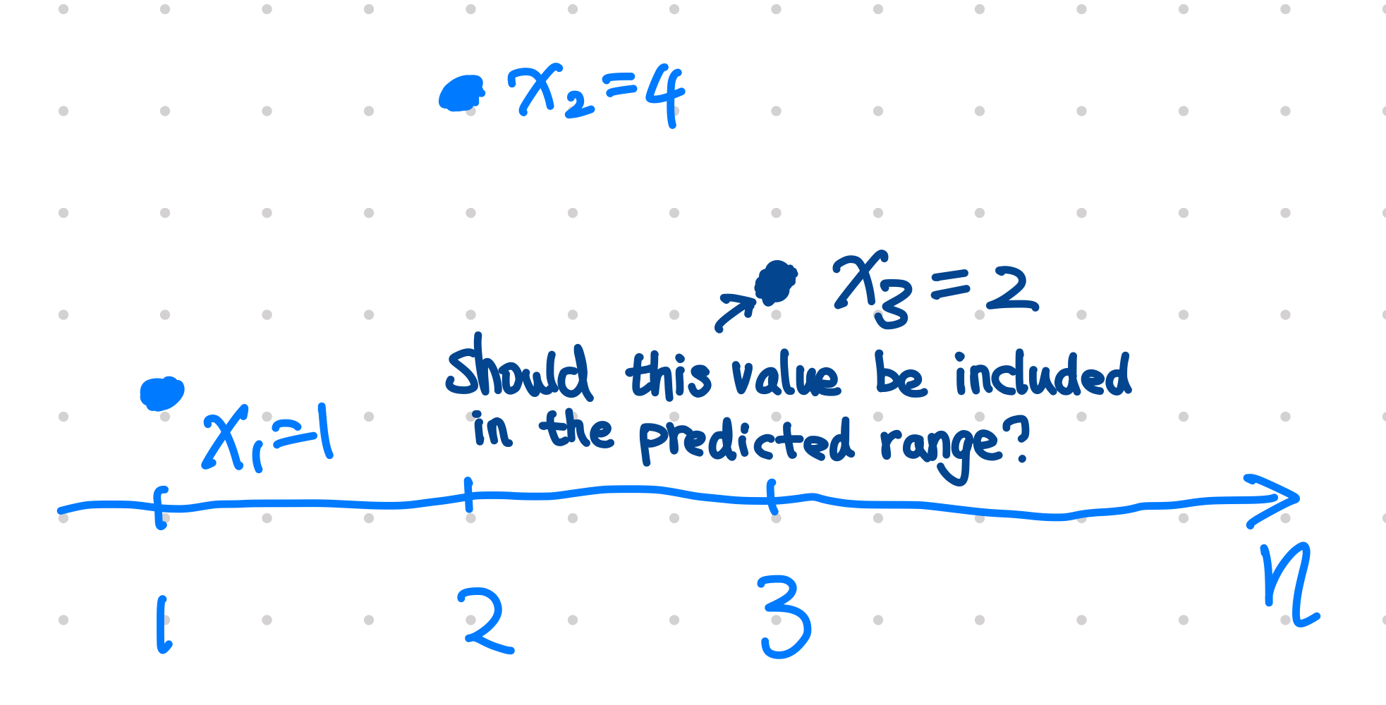
We have two existing datapoints and try to decide whether the third data point $x_3$ should be included in the predicted region with $\alpha=0.05$ significance level.
Given two existing data points
$$ B_3 = \{\{ x_1=1, x_2=4 \}\}, $$
we will decide if $x_3=2$ should be included in our predicted region of significance level $\alpha=0.05$.
To be able to test if $x_3=2$ falls inside the predicted region, we simply take the average of data points for the point prediction, and we use L1 norm as the nonconformity measure, i.e.,
$$ \begin{align} f(B_n) &= \frac{1}{n}\sum_i x_i \\ A(f(B_n), x) &= \lvert x - f(B_n) \rvert. \end{align} $$
With the model and nonconformity measure set, we can deicide whether the new data poin $x_3 = 2$ should be included in the predicted region of significance level $\alpha=0.05$.
For $i=1,2,3$,
calculate
$$ f_i = f(B_3\{\{x_i\}\}) $$
calculate the nonconformity measure
$$ \alpha_i = A(f_i, x_i) $$
With all $\alpha_i$, count all the data points that leads to $\alpha_i\geq \alpha_3$, denoted as $N_{\alpha_i\geq\alpha_3}$, calculate the probability
$$ p_x = \frac{N_{\alpha_i\geq\alpha_3}}{n}. $$
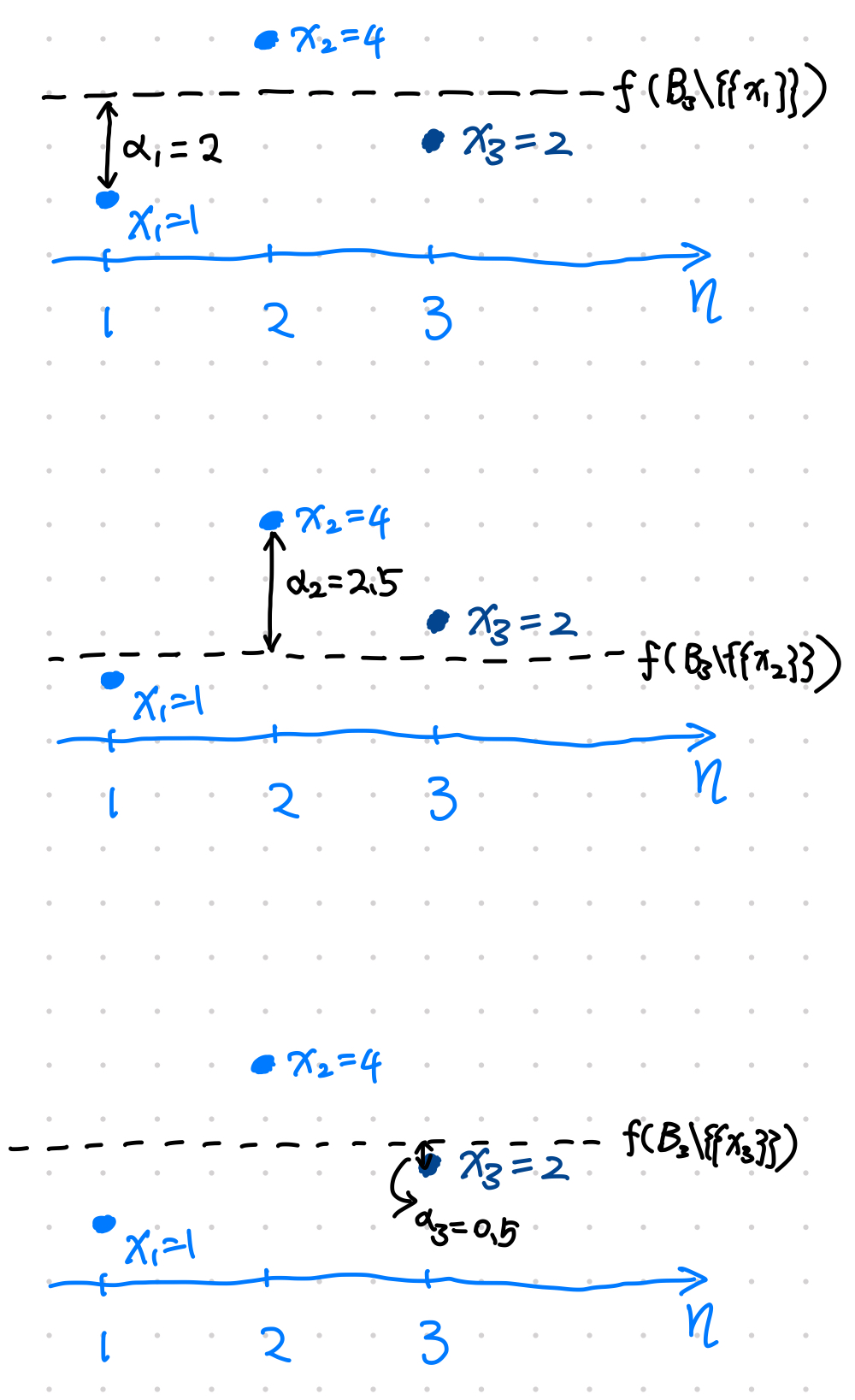
Steps to decide whether to include $x_3=2$ in the predicted region.
This algorithm is basically a hypothesis test procedure using the [[Neyman-Pearson theory]] Neyman-Pearson Theory The Neyman-Pearson hypothesis testing tests two hypothesis, hypothesis $H$, and an alternative hypothesis $H_A$. Neyman-Pearson Lemma The Neyman-Pearson Lemma is an very intuitive lemma to understand how to choose a hypothesis. The lecture notes from PennState is a very good read on this topic1. An example For simplicity, we assume that there exists a test statistic $T$ and $T$ can be used to measure how likely the hypothesis $H$ is true, e.g., the hypothesis $H$ is false, corresponds to $T$ … 1.
Requires Exchangeability
The algorithm assumes the data points are exchangeabile as we assume no statistical difference between
$$ x_1, x_2, x_3, ..., x_n, $$
and
$$ x_2, x_3, ..., x_n, x_1 $$
and
$$ x_1, x_3, ..., x_n, x_2 $$
and all the possible permutations of this pattern. Obviously, i.i.d. data satisfies this condition. Note that i.i.d. is a more stringent condition1.
Bonferroni Correction
For predictions involves multiple variable, we should consider the [[Bonferroni Correction]] Bonferroni Correction Bonferroni correction is very useful in a multiple comparison problem .
wiki/statistical-estimation/conformal-prediction:wiki/statistical-estimation/conformal-prediction Links to:L Ma (2022). 'Conformal Prediction', Datumorphism, 04 April. Available at: https://datumorphism.leima.is/wiki/statistical-estimation/conformal-prediction/.