Confidence Interval
Confidence interval is the interval that we are about a certain degree of confident that we have captured the true mean. From this point of view, the name confidence interval is rather misleading.
We will use upper cases for the abstract variable and lower cases for the actual numbers.
Why is Confidence Interval Needed?
Suppose I sample the population multiple times, the mean value $\mu_i$ of the sample is calculated for each sample. It is a good question to ask how different these $\mu_i$ are compared to the true mean $\mu_p$ of the population.
In this article, we would need to specify several notations.
- $X$ is the quantity we are measuring.
- $\bar X$ is the mean of the quantity $X$.
Confidence Interval
This theorem states that the probability for the true mean $\mu_p$ to fall into a specific range can be calculated using
$$ P( \mu_p \in [\bar X - z_{\alpha/2} \sigma_{\bar x}, \bar X + z_{\alpha/2} \sigma_{\bar x} ] ) = 1-\alpha. $$
Here $z_{\alpha/2}$ is the $z$ value which makes the probability to be in between $[-z_{\alpha/2}, z_{\alpha/2}]$ to be $1-\alpha$. As shown in the following figure. $\sigma_{\bar x}$ is the standard error of the mean for the sample.
- It is NOT the standard deviation of the sample data.
- It is NOT the population standard deviation.
- It is NOT the standard error calculated using only the sample data.
- It depends on the sample size. The larger the sample size, the smaller it will be.
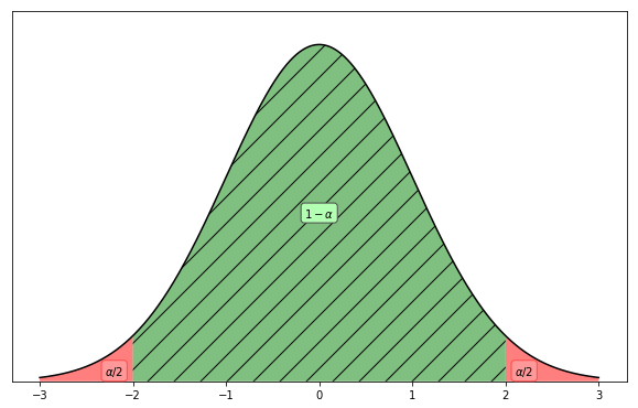
The definition of $\alpha$ for a normal distribution. In a probability distribution, the area under the curve should be 1. Or the integral of the curve from $-\infty$ to $\infty$ should be 1. $\alpha$ is the sum of the two red areas. In this example, we actually have $\alpha=0.05$.
The confidence level is a weird measurement of our statistical confidence.
Imagine we are drawing 100 samples from the population and calculate the range $[\bar X - z_{\alpha/2} \sigma_{\bar x}, \bar X + z_{\alpha/2} \sigma_{\bar x} ]$. We would have 100 different ranges. How many of them would actually contain the true mean? The answer is probably around $(1-\alpha)$ fraction of all the 100 calculations. When we have a huge amount of samples, this probability becomes quite faithful.
Why is this a representation of our confidence? Imagine we choose one sample from this 100 calculations. The probability that this specific number $[\bar X - z_{\alpha/2} \sigma_{\bar x}, \bar X + z_{\alpha/2} \sigma_{\bar x} ]$ (with all the numbers substituted using the sample values, for example $[-1,2]$, which is different from every other sample calculations) contains the true mean is also $(1-\alpha)$.
In other words, $[\bar X - z_{\alpha/2} \sigma_{\bar x}, \bar X + z_{\alpha/2} \sigma_{\bar x} ]$ is the interval that we are $1-\alpha$ confident that we have captured the true mean. From this point of view, the name confidence interval is rather misleading.
Be Professional and Call Them by the Names
- Confidence limits or fiducial limits is the range $[\bar X - z_{\alpha/2} \sigma_{\bar x}, \bar X + z_{\alpha/2} \sigma_{\bar x} ]$.
- $1-\alpha$ is the confidence coefficient
- $z_\alpha$ is the critical value.
What If the Confidence Limits is Huge Range?
As we are talking about the confidence limit, we would imagine it is different for different distributions even for the same $\alpha$.
If the confidence limits are large, it indicates that we won’t be able to pin down the true mean very well. In this case, our estimation is less precise.
Thus the width of the confidence limits
$$ \bar X + z_{\alpha/2} \sigma_{\bar x} - \left(\bar X - z_{\alpha/2} \sigma_{\bar x} \right) = 2 z_{\alpha/2} \sigma_{\bar x} $$
is a measure of the precision of our estimation, which is defined as twice of the margin of error, i.e.,
$$ 2 E = 2 z_{\alpha/2} \sigma_{\bar x}. $$
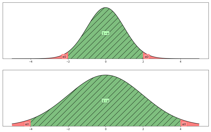
The larger the margin of error $E$, the harder to pin down the true mean. In the two panels, we have larger $E$ for the lower panel whose sample size is approximately 1/4 of the upper panel’s. This is trivial since smaller samples leads to larger $\sigma_{\bar x}$ thus wider distribution. In this example, we have $\alpha=0.05$.
What If We Don’t Know the Population Standard Deviation?
Wait a minute. To calculate $\sigma_{\bar x}$ we need the population standard deviation $\sigma_p$,
$$ \sigma_{\bar x} = \sigma_p/\sqrt{n}. $$
As we mentioned, this is NOT what you calculate using the sample data only.
For this problem, we have a macroscopic view and microscopic view.
Macroscopic View
As the population size approach infinity, we expect to recover the population distribution. Suppose we have a large sample size, it is good enough to use the estimation of the standard error $S_{\bar x}$ to represent the actual standard error $\sigma_{\bar x}$.
In this case, we
- calculate the standard deviation of the sample, $S$,
- estimate the standard error of the mean $S_{\bar x}$ using $S_{\bar x}=S/\sqrt{n}$ where $n$ is the sample size,
- use $S_{\bar x}$ instead of (the unknown) $\sigma_{\bar x}$ to calculate the scalar $z_{\alpha/2}$.
Basically, we assume that
$$ \frac{\bar X - \mu}{\sigma_{\bar x}} \sim \frac{\bar X - \mu}{ S_{\bar x} } $$
Microscopic View
When we have a small sample size, we do not have the macroscopic view to neglect the “glitches”.
We have been talking approximations
$$ \frac{\bar X - \mu}{\sigma_{\bar x}} \sim \frac{\bar X - \mu}{ S_{\bar x} } . $$
If this is not the case, then how good is the approximation? To answer this question, we need to know the distribution of $\frac{\bar X - \mu}{\sigma_{\bar x}}$. It is called t distribution. Since this distribution is known. We simply replace the assumed normal distribution of the sample mean using this t distribution. We will still have our confidence limits and confidence levels using this t distribution.
What Sample Size is Required for Macroscopic View?
If the sample size is larger than 30!
wiki/statistical-estimation/confidence-interval:wiki/statistical-estimation/confidence-interval Links to:L Ma (2019). 'Confidence Interval', Datumorphism, 01 April. Available at: https://datumorphism.leima.is/wiki/statistical-estimation/confidence-interval/.