Model Selection
Suppose we have a generating process that generates some numbers based on a distribution. Based on a data sample, we could reconstruct some sort of theoretical models to represent the actual generating process.
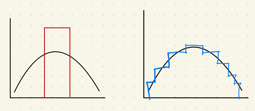
The black curve represent the generating process. The red rectangle is a very simple model that captures some major samples. The blue step-wise model is capturing more sample data but with more parameters.
In the above example, the red model on the left is not that good in most cases while the blue model seems to be better. In reality, the choice depends on the usage of the model. But we can already tell that the balance is between how well the model describes the data and how complicated the model is.
To make it even more conflicting, the following illustration shows another generating process and two corresponding models.
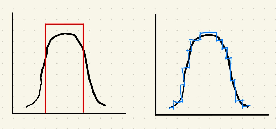
The black curve represent the generating process. The red rectangle is a very simple model that captures some major samples. The blue step-wise model is capturing more sample data but with more parameters.
In this case, we might agree that the red simple model is probably good enough for many situations. While the blue model is captures more features of the data, we have to deal with more parameters.
What is a Good Model?
Presumably, a good model should be
- plausibility (we do not like models that explain suicide rates primarily based on the coverage of Internet Explorer),
- balance of parsimony and goodness-of-fit (we can not use models that perform badly but a good-performing model with ten-thousand parameters is not exactly a good one either most of the time),
- coherence of the underlying assumptions,
- easy to understand when it breaks down,
- consistency with known results,
- especially with the simple and basic phenomena,
- ability to explain rather than describe data,
- extent to which model predictions can be falsified through experiments.
How to choose a model?
To choose a good model, we need a framework to compare two models. The comparison shall at least address the goodness-of-fit and parsimony.
Many methods have been proposed to deal with the balance between parsimony and goodness-of-fit, e.g.,
- Information criteria (IC) such as [[AIC]] Akaike Information Criterion Suppose we have a model that describes the data generation process behind a dataset. The distribution by the model is denoted as $\hat f$. The actual data generation process is described by a distribution $f$. We ask the question: How good is the approximation using $\hat f$? To be more precise, how much information is lost if we use our model dist $\hat f$ to substitute the actual data generation distribution $f$? AIC defines this information loss as $$ \mathrm{AIC} = - 2 \ln p(y|\hat\theta) + … and [[BIC]] Bayesian Information Criterion BIC considers the number of parameters and the total number of data records. ,
- Minimum description length ( [[MDL]] Minimum Description Length MDL is a measure of how well a model compresses data by minimizing the combined cost of the description of the model and the misfit. ),
- Bayes factors.
Here we demonstrate how IC can tell us which model is better. We calculate the IC of all the models at hand and specify the delta
$$ \Delta _i = \mathrm{IC}_i - \operatorname{min} \mathrm{IC}. $$
Then we specify the weights of models
$$ w_i = \frac{ \exp\{-\Delta_i/2\} }{ \sum_{m=1}^M \exp\{-\Delta_m/2\} }. $$
The model with larger weight $w_i$ is a better model.
There are other criteria too. For example, we can use the minimum description lengthor the Bayes factors.
wiki/model-selection/model-selection:wiki/model-selection/model-selection Links to:L Ma (2020). 'Model Selection', Datumorphism, 11 April. Available at: https://datumorphism.leima.is/wiki/model-selection/model-selection/.