Decision Tree

#Decision Tree #Supervised Learning #Statistical Learning #Basics

In this article, we will explain how decision trees work and build a tree by hand.

The code used in this article can be found in this repo.

Definition of the problem

We will decide whether one should go to work today. In this demo project, we consider the following features.

feature	possible values
health	0: feeling bad, 1: feeling good
weather	0: bad weather, 1: good weather
holiday	1: holiday, 0: not holiday

For more compact notations, we use the abstract notation $\{0,1\}^3$ to describe a set of three features each with 0 and 1 as possible values. In general, the notation $\{0,1\}^d$ indicates $d$ binary features.

Our prediction will be a binary result, 0 or 1, with 0 indicates staying at home and 1 indicates going to work.

To be compact, this prediction can be denoted as $\{0,1\}^1$.

How to Describe a Decision Tree

In theory, we would expect a decision tree of the following.

It is straight forward to prove that the max required depths and max required leaves of a model that maps $\{0,1\}^d$ to $\{0,1\}^1$ are $d+1$ and $2^d$. In our simple example, some of the branches are truncated based on our understanding of the problem. In principle, the branch “feeling bad” could also go on to the next level.

Data

However, we do not forge trees using experience. We build the tree using data.

The following is a sample of the full dataset.

	health	weather	holiday
0	0	0	1
1	1	1	1
2	1	0	1
3	0	0	0
4	1	0	1

Full Data

	health	weather	holiday	go_to_office
0	0	0	1	0
1	1	1	1	0
2	1	0	1	0
3	0	0	0	0
4	1	0	1	0
5	0	1	0	0
6	0	1	1	0
7	1	1	0	1
8	0	1	0	0
9	0	0	1	0
10	0	0	1	0
11	0	0	1	0
12	1	0	0	0
13	1	0	0	0
14	0	0	1	0
15	0	0	1	0
16	0	1	0	0
17	0	1	0	0
18	0	1	1	0
19	0	1	1	0
20	1	1	1	0
21	0	0	1	0
22	1	0	1	0
23	1	1	1	0
24	0	0	0	0
25	0	0	1	0
26	1	0	0	0
27	0	1	1	0
28	1	0	0	0
29	1	0	1	0
30	1	0	1	0
31	0	0	0	0
32	0	0	0	0
33	1	1	1	0
34	1	1	1	0
35	1	0	0	0
36	1	1	1	0
37	0	1	1	0
38	0	1	1	0
39	1	1	1	0
40	0	0	1	0
41	0	1	1	0
42	1	0	0	0
43	1	0	0	0
44	1	1	1	0
45	0	0	1	0
46	0	0	1	0
47	1	0	1	0
48	0	1	0	0
49	1	0	1	0
50	1	1	0	1
51	0	0	1	0
52	1	0	0	0
53	1	0	1	0
54	1	0	1	0
55	0	0	1	0
56	0	0	0	0
57	0	1	0	0
58	1	1	1	0
59	1	0	1	0
60	1	1	1	0
61	0	1	0	0
62	0	1	1	0
63	0	0	0	0
64	0	1	0	0
65	1	0	1	0
66	0	1	1	0
67	1	1	0	1
68	0	0	0	0
69	1	0	0	0
70	0	0	0	0
71	0	0	1	0
72	0	0	1	0
73	0	0	1	0
74	0	0	0	0
75	0	1	1	0
76	1	1	1	0
77	1	1	0	1
78	0	1	0	0
79	0	0	0	0
80	0	0	0	0
81	1	0	0	0
82	0	1	0	0
83	0	1	0	0
84	0	1	0	0
85	0	0	0	0
86	1	1	1	0
87	1	0	0	0
88	0	1	0	0
89	1	1	1	0
90	1	1	0	1
91	1	0	0	0
92	0	1	1	0
93	0	0	0	0
94	1	1	0	1
95	1	0	1	0
96	0	0	1	0
97	0	1	1	0
98	1	0	0	0
99	1	1	0	1

Build a Tree

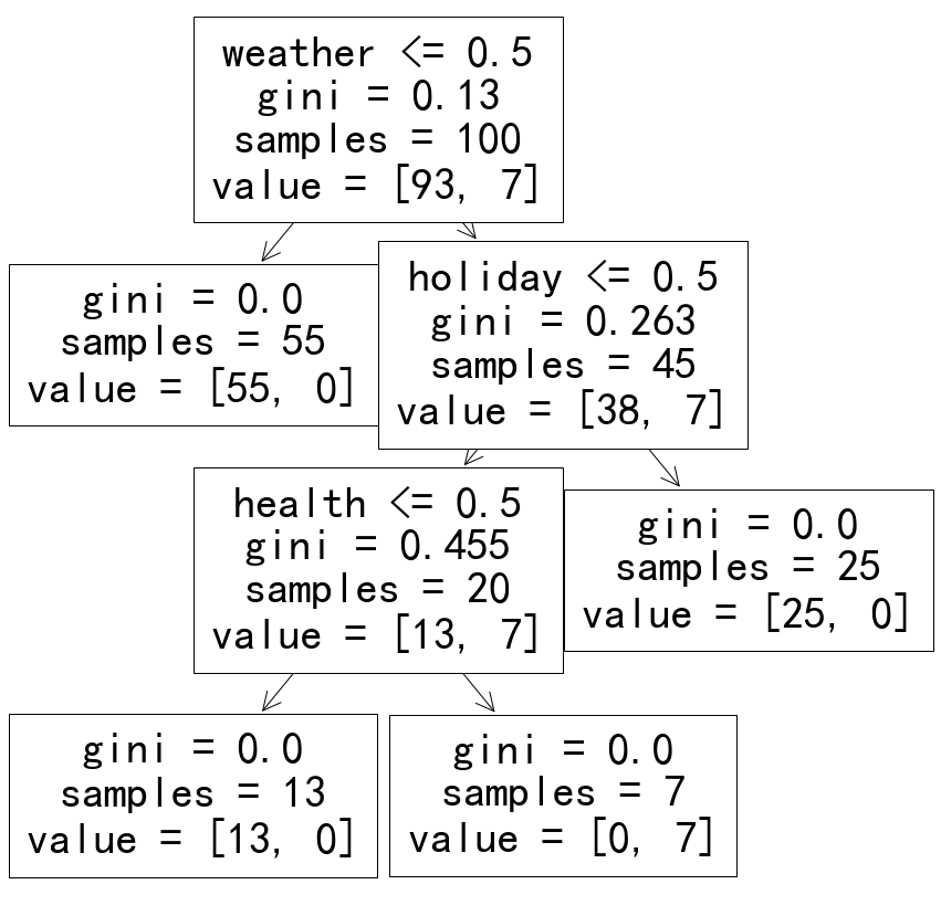
A decision tree trained with the dataset.

Reading the Decision Tree Chart

On each node of the tree, we read loads of information.

We will look into the root node as an example. The feature name and value range are denoted on the first row, i.e., weather<= 0.5, which means that we are making decisions based on whether the value of the weather feature less or equal to 0.5. If the value is less or equal to 0.5, we go the left branch, otherwise, we go to the right branch. The following rows in the node are assuming the condition is satisfied.

On the second row, we read the gini impurity value. Gini impurity is a measure of the impurity of the data under the condition.

On the third row, samples of the given condition (weather <= 0.5) is also given.

Finally, we read the values of the samples. In this example, value = [93, 7], i.e., 93 of the samples have target value 0, 7 of the samples have target value 1.

This is a very good result. It is the same as our theoretical expectations.

Surely it will. We forged the dataset based on the theoretical expectations.

Here is an example of using data that doesn’t always fit into our theoretical model.

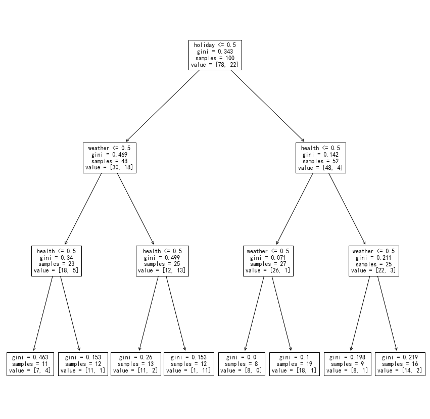
A decision tree trained with a fake “impure dataset” that doesn’t always fit into our theoretical model."

Overfitting

Fully grown trees will most likely to overfit the data since they always try to grow pure leaves. Besides, fully grown trees grow exponentially as the number of features grow which requires a lot of computation resources.

Applying Occam’s razor, we prefer smaller trees as long as the trees can explain the data well.

To achieve this, we will either have to limit how the trees grow during training, or pruning the trees after the trees are built.

Pruning of a tree is achieved by replacing subtrees at a node with a leaf if some certain conditions based on cost estimations.

Remarks

The Iterative Dichotomizer 3 algorithm, aka ID3 algorithm, is one of the most famous implementations of the decision tree. The following is the “flowchart” of the algorithm.

graph TD Leaf("Prepare samples in node") MajorityVote["Calculate majority vote"] Assign[Assign label to node] Leaf --> MajorityVote --> Assign Assign --> Split1[Split on feature 1] Assign --> Splitdots["..."] Assign --> Splitd[Split on feature d] subgraph "split on a subset of features" Split1 --> |"Split on feature 1"|B1["Calculate gain of split"] Splitdots --> |"..."| Bdots["..."] Splitd --> |"Split on feature d"| Bd["Calculate gain of split"] end B1 --> C["Use the split with the largest gain"] Bdots --> C Bd --> C C --> Left["Prepare samples in left node"] C --> Right["Prepare samples in right node"] subgraph "left node" MajorityVoteL["Calculate majority vote"] AssignL(Assign label to left node) Left --> MajorityVoteL --> AssignL end subgraph "right node" MajorityVoteR["Calculate majority vote"] Right --> MajorityVoteR AssignR(Assign label to right node) MajorityVoteR --> AssignR end

To “calculate the gain of the split”, we use information gain or Gini impurity.

Planted: 2019-12-25 by L Ma;

References:

Shalev-Shwartz, S., & Ben-David, S. (2013). Understanding machine learning: From theory to algorithms. Understanding Machine Learning: From Theory to Algorithms.

Supplementary:

Python code used in this article

Dynamic Backlinks:

Random Forest

random forest in machine learning

Gini Impurity

The Gini impurity is a measurement of the impurity of a set.

Information Gain

The information is a measurement of the entropy of the dataset.

Curriculum

The path that I follow

Links to: