Neural ODE

#Deep Learning #Neural ODE

In [[neural networks]] Artificial Neural Networks Simple artificial neural networks using multilayer perceptron , residual connections is a popular architecture to build very deep neural networks¹. Apart from residual networks, there are many other designs for deep neural networks²³⁴⁵⁶. These methods share similar ideas that the layered structure in deep neural networks can be treated as a dynamical system and these different architectures are different numerical approaches of solving the dynamical system.

Figure taken from He K, Zhang X, Ren S, Sun J. Deep Residual Learning for Image Recognition. arXiv [cs.CV]. 2015. Available: http://arxiv.org/abs/1512.03385

The degradation problem

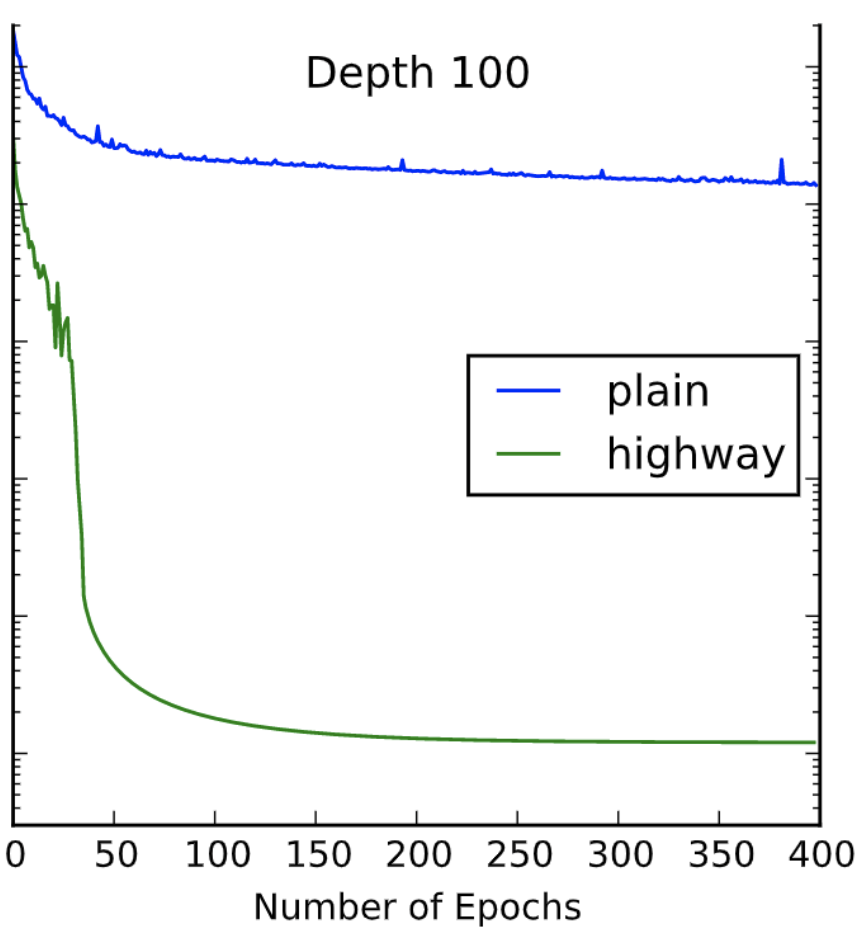
For deep neural networks, not all deep architectures are able to produce results that are significantly better than shallow architectures. It has been observed that “simply” stacking more layers to a shallow network may reach some saturated performance quite fast and leaving most of the added layers less useful.

In the work by Srivastava et al, they showed a comparison of “plain” deep networks, which has the layers simply stacked, and their highway networks which has gates that control how close to identity each layer is. The following is a figure extracted from their seminal work Highway Networks.

Highway Networks

Neural ODE

An alternative view of the above approaches as [[Ordinary Differential Equations]] Ordinary Differential Equations Solving ODEs Using Finite Difference Methods of dynamical system. For example, a residual connection structure can be reformulated as a first order different equation⁷, i.e., a residual connection of the following form

$$ h_{t+1} = h_t + f(h_t, \theta_t), $$

is a discretized case of the differential equation

$$ \frac{\mathrm d h(t)}{\mathrm d t} = f(h(t), \theta(t), t). $$

In the above equation, the variable $t$ is not necessarily physical time. This is an “extrapolated” version of the number of layers. But under some certain problems, $t$ can be the physical time.

For simplicity, we can even assume a set of static parameters $\theta$.

Given any Jacobian $f(h(t), \theta(t), t)$, we can, at least numerically, perform integration to find out the value of $h(t)$ at any $t=t_N$,

$$ h(t_N) = \int_{t_0}^{t_i} f(h(t), \theta(t), t) \mathrm dt. $$

In this formalism, we find out the transformed input $h(t_0)$ by solving this differential equation. In traditional neural networks, we achieve this by stacking many layers of neural networks using skip connections.

In the original Neural ODE paper, the authors used the so-called reverse-model derivative method⁷.

Time Series and Neural ODE

We can model the data generating process behind time series data using dynamical systems. The simplest continuous formulation is a first order ordinary differential equation. Given time series $\{y_i\}$, we can use the following first order differential equation

$$ \frac{\mathrm dy(t)}{\mathrm d t} = f(y(t), \theta, t). $$

Generally speaking, finding $f$ requires a lot of hypothesis and explorations. Neural ODE provides a general framework to approximate such a dynamical system.

For example, we can feed some data points $\{(t_0, y_0), (t_1, y_1), \cdots, (t_m, y_m)\}$ into the model, and we solve the differential equation for $t=t_{m+1}$. By calculating the loss and applying backpropagation, we can optimize the parameters $\theta$ in the Jacobian $f$. We then feed the next data points $\{(t_1, y_1), (t_2, y_2), \cdots, (t_{m+1}, y_{m+1})\}$ and solving for $t=t_{m+2}$ and do the same. By exhausting the whole dataset, we can find an “optimal” Jacobian $f$ which can be used in inference to rebuild the whole dynamics.

Planted: 2022-08-13 by L Ma;

References: