Restricted Boltzmann Machine
This article uses Mehta2018 extensively.
Latent variables introduce extra correlations between the nodes in a network. Introducing hidden units can also help us remove the direct connection between some nodes in a Boltzmann machine and create a restricted Boltzmann machine. A restricted Boltzmann machine requires less computation while having some expressing power.
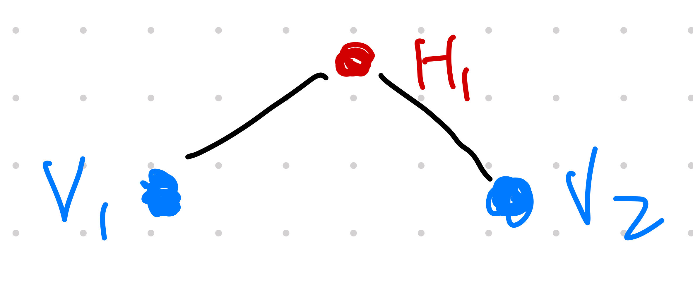
Given Ising like interactions between the nodes, flipping node V1 is likely to also flip node V2 as they are connected through hidden unit H1. They are correlated. Removing the hidden unit leaves us two uncorrelated units.
The Ising Model
Given a Ising-like energy function (c.f. [[MaxEnt Model]] MaxEnt Model Maximum Entropy models makes least assumption about the data )
$$ E(x) = - \sum_i h_i x_i - \frac{1}{2} \sum_{ij} J_{ij} x_i x_j, $$
The term $\sum_{ij} J_{ij} x_i x_j$ can be decomposed using the [[Cholesky Decomposition]] Cholesky Decomposition Decomposing a matrix into two Cholesky decomposition,
$$ \sum_{ij} J_{ij} x_i x_j = \sum_{ijk} W_{ik} W_{kj}^T x_i x_j = \sum_{ijk} W_{ik} W_{jk} x_i x_j. $$
The energy function can be rewritten as
$$ E(x) = - \sum_i h_i x_i - \frac{1}{2} \sum_{ijk} W_{ik} W_{jk} x_i x_j. $$
The distribution (derived using [[the Max Entropy principle]] MaxEnt Model Maximum Entropy models makes least assumption about the data ) is
$$ \begin{equation} p(x) \propto \exp{ \left( \sum_i h_i x_i + \frac{1}{2} \sum_{ijk} W_{ik} W_{jk} x_i x_j \right)} \label{eqn-boltzmann-dist-hopfield} \end{equation} $$
Latent Variables: From Energy Function to Distribution
Using the [[the Hubbard-Stratonovich Identity]] The Hubbard-Stratonovich Identity Very useful in calculating the partition function , we transform equation $\eqref{eqn-boltzmann-dist-hopfield}$ into1
$$ \begin{align} p(x) \propto & \exp{\left( \sum_i h_i x_i \right)} \exp{ \left(\frac{1}{2} \sum_{ijk} W_{ik} W_{jk} x_i x_j \right)} \\ \propto & \exp{\left( \sum_i h_i x_i \right)} \frac{1}{\sqrt{2\pi}} \int \mathrm dh_k\, \exp{ \sum_k \left( -\frac{1}{2} h_k^2 + \sum_i x_i W_{ik} h_k \right)} \\ \propto & \frac{1}{\sqrt{2\pi}} \int \mathrm dh_k\, \exp{ \left[ \sum_i h_i x_i + \sum_k \left( -\frac{1}{2} h_k^2 + \sum_i x_i W_{ik} h_k \right) \right]}. \end{align} $$
Define a new energy function
$$ \tilde E(x,h) = - \sum_i h_i x_i - \sum_k \left( -\frac{1}{2} h_k^2 + \sum_i x_i W_{ik} h_k \right) . $$
The distribution becomes the marginalization of the hidden variable
$$ \begin{equation} p(x) \propto \int \mathrm dh\, \exp{ \left( -\tilde E(x,h) \right) }. \label{eqn-marginalization-new-energy-function} \end{equation} $$
Use the result $\eqref{eqn-marginalization-new-energy-function}$, we can define a model with two groups of nodes $x$ and $h$. The group $x$ has no internal connections, i.e., no high order correlations like $x^2$. The group of nodes $x$ is called visible layer while the hidden nodes $h$ are called hidden layer. In general, we require a form of energy
$$ \tilde E(x, h) = -\sum_i a_i(x_i) - \sum_k b_k(h_k) - \sum_{ik} x_i W_{ik} h_k. $$
Usually, we use the form
$$ \begin{equation} \tilde E(x, h) = -\sum_i a_i x_i - \sum_k b_k h_k - \sum_{ik} x_i W_{ik} h_k, \label{eqn-energy-function-with-latent-variables} \end{equation} $$
with the nodes can only be 0 or 1. The visible layer and hidden layer are called Bernoulli as they have binary states.
Latent Variables: From Distribution to Energy Function
We can also derive the energy function for distributions of the form $\eqref{eqn-energy-function-with-latent-variables}$. For easier understanding, we define a new joint distribution $p(x, h)$ from
$$ p(x, h) = \frac{\exp{\left( -\tilde E(x, h) \right)}}{Z}, $$
so that
$$ p(x) = \int \mathrm d h\, p(x, h) = \frac{ \exp{\left( -E(x) \right)} }{Z}. $$
Using the above two definitions, we have
$$ \exp{\left(-E(x)\right)} = \int \mathrm d h \, \exp{\left( -\tilde E(x, h) \right)}, $$
from which we derive a formalism for the marginalized energy function
$$ \begin{align} E(x) =& - \ln \int \mathrm d h \, \exp{\left( -\tilde E(x, h) \right)} \\ =& \sum_i a_i(x_i) - \sum_k \ln \int \mathrm d h_k \, \exp{\left( b_k(h_k) \right)} \exp{\left( \sum_j x_j W_{jk}h_k \right)}. \label{eqn-e-x} \end{align} $$
This energy function can be expanded using the cumulant2, we can decompose the energy function $E(x)$, equation $\eqref{eqn-e-x}$,
$$ E(x) = -\sum_i a_i(x_i) - \sum_i \sum_k \kappa^{(1)}_k W_{ik} x_i - \frac{1}{2}\sum_{ij} \left( \sum_{k} \kappa^{(2)}_k W_{ik} W_{jk} \right) x_i x_j + \cdots $$
where $\kappa^{(\cdot)}$ are coefficients related to the cummulant3. We can find any order of correlations even without in-group connections between the visible nodes.
Gradient of Log-likelihood
In this section, we will focus on Bernoulli layers, i.e., $a_i(x_i) = a^0_i x_i$ and $b_k(h_k) = b^0_k h_k$
Using the results from [[MaxEnt model]] MaxEnt Model Maximum Entropy models makes least assumption about the data , we can find the gradient of the log-likelihood $\mathcal L(W_{ik}, a_i, b_k)$,
$$ \begin{align} \partial_{W_{ik}} \mathcal L =& \langle x_i h_k \rangle_{\text{model}} - \langle x_i h_k \rangle_{\text{data}} \\ \partial_{a^0_i} \mathcal L =& \langle x_i \rangle_{\text{model}} - \langle x_i \rangle_{\text{data}} \\ \partial_{b^0_k} \mathcal L =& \langle h_k \rangle_{\text{model}} - \langle h_k \rangle_{\text{data}}. \end{align} $$
The calculation of $\langle \cdot \rangle_{\text{model}}$ is easier in RBM.
For [[first order Markov chains]] State Space Models The state space model is an important category of models for sequential data such as time series , the visible units do not depend on themselves as there are not direct connections between the visible units. So are the hidden units. That being said, we have $p(x\mid h)$ and $p(h\mid x)$.
In this simple situation, the distributions can be sampled using [[Gibbs sampling]] Gibbs Sampling Gibbs sampling is a sampling method for Bayesian inference and MCMC . To calculate $p(h\mid x)$, we will clamp our visible units to the data values then infer $h$ which will be used to infer $x$ based on $p(x\mid h)$. Iterate this process we will be able to sample the model, i.e.,
$$ \begin{align*} & p(h\mid x_0) \to h_0 \\ \Rightarrow & p(x\mid h_0) \to x_1 \\ \Rightarrow & p(h\mid x_1) \to h_1 \\ \Rightarrow & \cdots \end{align*} $$
Hubbard1959 Hubbard J. Calculation of Partition Functions. Physical Review Letters. 1959. pp. 77–78. doi:10.1103/physrevlett.3.77 ↩︎
Cumulant Contributors to Wikimedia projects. Cumulant. In: Wikipedia [Internet]. 7 May 2021 [cited 18 Jun 2021]. Available: https://en.wikipedia.org/wiki/Cumulant ↩︎
Mehta2018 Mehta P, Bukov M, Wang C-HH, Day AGRR, Richardson C, Fisher CK, et al. A high-bias, low-variance introduction to Machine Learning for physicists. Phys Rep. 2018;810: 122. doi:10.1016/j.physrep.2019.03.001 ↩︎
- Mehta2018 Mehta P, Bukov M, Wang C-HH, Day AGRR, Richardson C, Fisher CK, et al. A high-bias, low-variance introduction to Machine Learning for physicists. Phys Rep. 2018;810: 122. doi:10.1016/j.physrep.2019.03.001
- Hubbard1959 Hubbard J. Calculation of Partition Functions. Physical Review Letters. 1959. pp. 77–78. doi:10.1103/physrevlett.3.77
- Cumulant Contributors to Wikimedia projects. Cumulant. In: Wikipedia [Internet]. 7 May 2021 [cited 18 Jun 2021]. Available: https://en.wikipedia.org/wiki/Cumulant
wiki/machine-learning/energy-based-model/restricted-boltzmann-machine:wiki/machine-learning/energy-based-model/restricted-boltzmann-machine Links to:L Ma (2021). 'Restricted Boltzmann Machine', Datumorphism, 06 April. Available at: https://datumorphism.leima.is/wiki/machine-learning/energy-based-model/restricted-boltzmann-machine/.