Confusion Matrix (Contingency Table)
Confusion Matrix
It is much easier to understand the confusion matrix if we use a binary classification problem as an example. For example, we have a bunch of cat photos and the user labeled “cute or not” data. Now we are using the labeled data to train a cute-or-not binary classifier.
Then we apply the classifier on the test dataset and we would only find four different kinds of results.
| Labeled as Cute | Labeled as Not Cute | |
|---|---|---|
| Classifier Predicted to be Cute | True Positive (TP) | False Positive (FP) |
| Classifier Predicted to be Not Cute | False Negative (FN) | True Negative (TN) |
This table is easy enough to comprehend. We have discussed the Type I and Type II errors in Types of Errors in Statistical Hypothesis Testing . Here False Positive (FP) is Type I error and False Negative (FN) is Type II error.
Then we loop through all cats in the test dataset, find the results and put the numbers in the table.
There are a few things to look at whenever we have a table. First things first, we would like to know the sum of each row and columns.
- The sum of the row “Classifier Predicted to be Cute” tells us the total number of cats classified as cute, aka, Total Predicted Positives (PP);
- The sum of the row “Classifier Predicted to be Not Cute” tells us the total number of cats classified as not cute, aka, Total Predicted Negatives (PN);
- The sum of the column “Labeled as Cute” tells us the total number of cats labeled as cute in the test dataset, aka, Total Positives (P);
- The sum of the column “Labeled as Not Cute” tells us the total number of cats labeled as not cute in the test dataset, aka, Total Negatives (N).
- The sum of the diagonal elements tells us the total number of cases where the classifier classified the data correctly.
Measures Defined
Property of the Dataset itself
Apart from these trivial properties about the test dataset defined above, we can define the Prevalence:
$$ \frac{ \text{ Total Positives } }{ \text{ Total Sample, or Total Positives + Total Negatives} } = \frac{ \text{ Labeled as Cute } }{ \text{ All Cats, or Labeled as Cute + Labeled as Not Cute} } $$
Performance of Classifier
We could define some quite general measures.
- Accuracy: $$\frac{ \text{ TP + TN } }{ \text{P + N} }$$
Now we recalculate the confusion matrix by dividing the values by some certain sums.
Confusion Matrix divided by the Column Sums
As mentioned in the previous sections, the sum of the columns are P (Total Positives) and N (Total Negatives). Dividing each column by the sum of the corresponding column gives us the prediction rate for each labels.
| Labeled as Cute | Labeled as Not Cute | |
|---|---|---|
| Classifier Predicted to be Cute | True Positive Rate (aka Recall) = TP/P | False Positive Rate = FP/N |
| Classifier Predicted to be Not Cute | False Negative Rate = FN/P | True Negative Rate (aka Specifity) = TN/N |
There are a few names to be emphasized.
- Recall: True Positive Rate
Confusion Matrix divided by the Row Sums
As mentioned, the sum of the rows indicates the
| Labeled as Cute | Labeled as Not Cute | |
|---|---|---|
| Classifier Predicted to be Cute | Positive Predictive Value (aka Precision) = TP/PP | False Discovery Rate = FP/PP |
| Classifier Predicted to be Not Cute | False Omission Rate = FN/PN | Negative Predictive Value = TN/PN |
There are a few names to be emphasized.
- Precision: Positive Predictive Value
Ratios, Scores, and More
We also have some other definitions of ratios, please refer to the bottom left corner of the table on the corresponding Wikipedia page linked in the references.
We will only define the F1 score ($\mathrm F_1$) here. As a F-measure,
$$ \begin{align} F_1 &= \frac{2}{ 1/\mathrm{Pression} + 1/\mathrm{Recall} } \\ & = \frac{2}{ \frac{PP}{TP} + \frac{P}{TP} } \\ & = \frac{2}{ \frac{PP+P}{TP} } \\ & = \frac{2}{ \frac{ (TP + FP) + (TP + FN) }{TP} } \\ & = \frac{1}{ 1 + \frac{ (FP + FN) }{2TP} } \end{align} $$
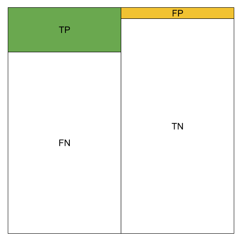
Confused by the Names?
There is a nice chart on this Wikipedia page.
The different metrics can be visualized using color blocks. We use green to represent the amount of TP, orange to represent the amount of FP.
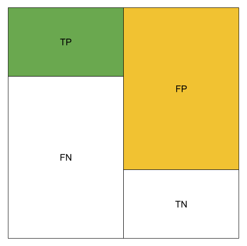
Low TP Rate;High FP Rate; Low Precision; Low Accuracy; Low Recall; Low F1
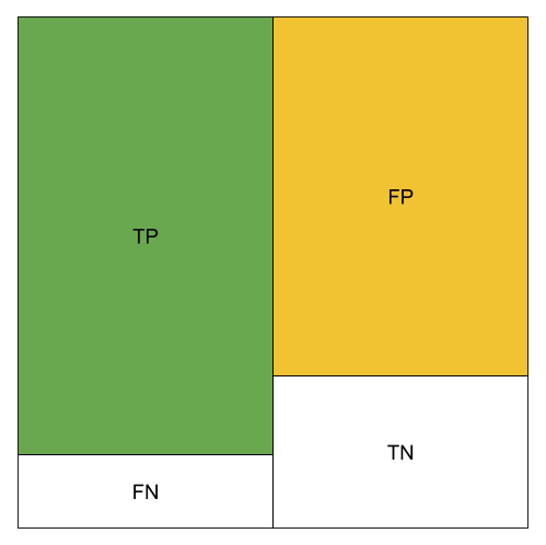
High TP Rate;High FP Rate; Not so good Precision; Not so good Accuracy; High Recall; Not so good F1
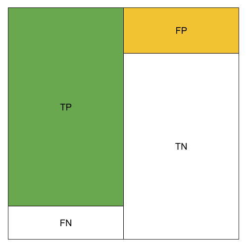
High TP Rate;Low FP Rate; Good Precision; Good Accuracy; High Recall; Good F1
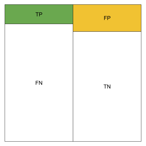
Low TP Rate;Low FP Rate; Low Precision; Low Accuracy; Low Recall; Low F1
Low TP Rate;Low FP Rate; High Precision; Low Accuracy; Low Recall; Low F1
wiki/machine-learning/basics/confusion-matrix:wiki/machine-learning/basics/confusion-matrix Links to:L Ma (2019). 'Confusion Matrix (Contingency Table)', Datumorphism, 05 April. Available at: https://datumorphism.leima.is/wiki/machine-learning/basics/confusion-matrix/.