Finite Element Method
Differential equations are fun!
Differential Equations and Boundary Conditions
Two Types of Boundary Conditions
As an example, we have a partial differential equation
$$ \frac{d^2u}{dx^2} + f = 0, $$
which describes a 1D problem.
- Dirichlet boundary condition: specify values for $u$, such as $u(0)=u_0$ and $u(L)=u_L$;
- Neumann boundary condition: specifiy values for $u_{,x}$.
If we have only Neumann boundary condition, the solution is not unique. One example for it is tossing a bar, which can have both Neumann BC at both ends but it is moving.
Example Problems
Elasticity Problem
We consider the displacement $u(x)$ at each space coordinate $x$ of a elastic bar under some external force. The strain is proportional to $u_{,x}$. The equation would be
$$ -\frac{d\sigma}{dx} = f. $$
Heat Transfer
Define temperature on a bar at each point $u(x)$. Heat transfer is proportional to the head gradient, $j= - \kappa u_{,x}$. The equation would be
$$
- \frac{dj}{dx} = f. $$
Strong Form and Weak Form of PDE
The strong form of differential equations is the original form we write down. The strong form requires each term to be well defined at each point. However, we can derive a weak form that requires each part to be well defined through the whole domain only, which is a relaxed requirement.
Galerkin Method
Suppose we need to find the solution to the equation
$$ \mathcal L_{x} \psi(x) = f(x). $$
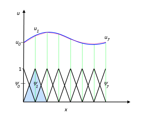
The key is that the solution can be approximated by
$$ \psi(x) = \sum_i u_i \phi_i(x), $$
where $\phi_i(x)$ are the basis functions.
The purpose is to find the the coefficients $u_i$. Galerkin method has three steps.
- discretize the space $x$ and function space: triangulation,
- discretize the function using the weak form: assembly,
- error estimation.
Triangulation is basically setting up the basis function in a discretized space $x$. One of the choicesis the hat function.
Triangulation from comsol multiphysics.
At each point $x$, there is a hat function responsible for the approximation within $[x-\Delta x, x+\Delta x]$.
Those hat functions forms the basis for the approximated solution
$$ \psi = \sum_i u_i \phi_i. $$
With this approximation, it requires the test function $v$ to write down the weak form. Basically we multiply $v$ on both sides of the equation then integrate by step. Then the differential equation can be rewrite into matrix form with basis $\phi_i$,
$$ \mathbf K \mathbf U = \mathbf L. $$
We solve the coefficients $\mathbf U$ from the matrix equation.
Collocation Method
This method is named collocation method because it employs two sets of basis functions.
To be specific, the result function should be
$$ \psi = \psi(x_0) + \sum_i U_i H_i(x) + \sum_i U’_i S_i(x), $$
where $\psi(x_0)$ takes care of the boundary condition at $x_0$.
With two set of basis functions the matrix form of the equation is double sized.
L Ma (2018). 'Finite Element Method', Datumorphism, 11 April. Available at: https://datumorphism.leima.is/wiki/dynamical-system/finite-element-method/.